Day 1: data input, manipulation and output

Jerry Davison and Martin Morgan

____________________________________________________________________________________________

Contents

1 Introduction to R
 1.1 R’s capabilities
 1.2 Resources for beginners
2 Using RStudio
 2.1 Help
3 Simple expressions
4 Input
5 Manipulation
6 Data types
7 Output

_______________________________________________________________________________________________

1 Introduction to R

R is an open-source statistical programming language. It is used to manipulate data, to perform statistical analyses, and to present graphical and other results. R consists of a core language, additional ‘packages’ distributed with the R language, and a very large number of packages contributed by the broader community. Packages add specific functionality to an R installation. R has become the primary language of academic statistical analyses, and is widely used in diverse areas of research, government, and industry.

R has several unique features. It has a surprisingly ‘old school’ interface: users type commands into a console; scripts in plain text represent work flows; tools other than R are used for editing and other tasks. R is a flexible programming language, so while one person might use functions provided by R to accomplish advanced analytic tasks, another might implement their own functions for novel data types.

As a programming language, R adopts syntax and grammar that differ from many other languages: objects in R are ‘vectors’, and functions are ‘vectorized’ to operate on all elements of the object; R objects have ‘copy on change’ and ‘pass by value’ semantics, reducing unexpected consequences for users at the expense of less efficient memory use; common paradigms in other languages, such as the ‘for’ loop, are encountered much less commonly in R.

Many authors contribute to R, so there can be a frustrating inconsistency of documentation and interface. R grew up in the academic community, so authors have not shied away from trying new approaches. Common statistical analyses are very well-developed.

1.1 R’s capabilities

‘Base’ R provides:

Additional packages provide:

1.2 Resources for beginners

_______________________________________________________________________________________________

2 Using RStudio

The RStudio application provides a convenient and flexible environment for your work with R. Figure 1 presents a view of a typical RStudio session.

See http://www.rstudio.com/ide for documentation and downloads for offline work on Linux, Windows and MAC systems.


PIC

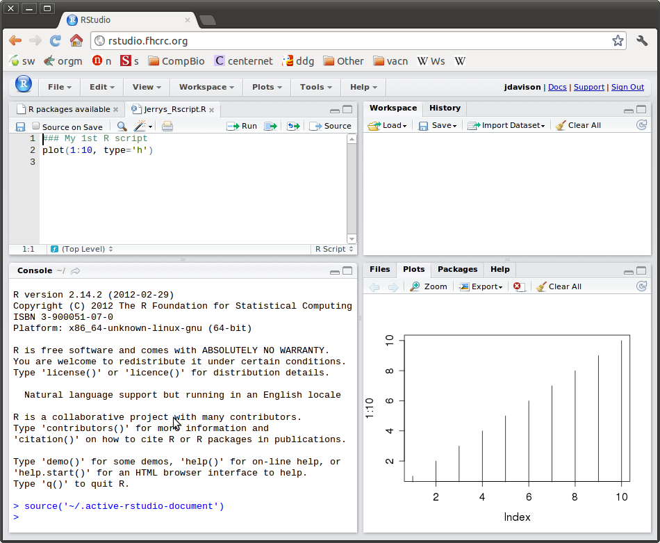
Figure 1: Typical RStudio configuration.

2.1 Help

R comes with extensive help. In RStudio, click the ‘help’ menu and choose ‘R help’. Important sections include

Search Engine and Keywords
is a convenient way to find help on what particular functions do; also try ? followed by a function name on the command line, e.g., ?read.table.
An Introduction to R
provides a thorough introduction to the language and key functions in R; consult this after becoming comfortable with the exercises we’ve gone through today.
R Data Import / Export
especially section 2 can be helpful when trying to get data in to R.

When not using RStudio, start the help system by typing the command help.start(). The R web site provides many useful links. Once you are comfortable with R, the R-help mailing list can be a very useful source of information, as can general-purpose forums like StackOverflow.

_______________________________________________________________________________________________

3 Simple expressions

R is a quite sophisticated system for data analysis, but that doesn’t mean it’s not comprehensible to beginners. Let’s start using it:

  > 2

  [1] 2

  > 2 + 2

  [1] 4

  > 2^10

  [1] 1024

One supported data type is the vector, specified in this way:

  > c(2, 4, 3)

  [1] 2 4 3

  > mean(c(2, 4, 3))

  [1] 3

  > sd(c(2, 4, 3))

  [1] 1

Data objects can be given names in an assignment statement:

  > x = c(2, 4, 3)
  > y = 2 + 2
  > x/y

  [1] 0.50 1.00 0.75

Exercise: evaluate these expressions: y/x, x-2/10, (x-2)/10

_______________________________________________________________________________________________

4 Input

Spreadsheet applications and R complement each other in that the former can provide nicely formatted columns, colored headers and convenient scrolling while R provides functional flexibility. You can access Excel worksheets and other table-like data files with R, and use R to write files readable by spreadsheets – R reads and writes tables written in comma- or tab-separated values formats.

We’ll first read the table ALLannotationFromExcel.txt that contains ALL (acute lymphoblastic leukemia) patient information:

  > filename = file.choose() # Go to the data directory to get the file
  > info = read.delim(filename)
  > ?read.delim

Then use R functions that tell us about the file:

  > class(info)

  [1] "data.frame"

  > colnames(info)

   [1] "id"             "diagnosis"      "sex"            "age"            "BT"
   [6] "remission"      "CR"             "date.cr"        "t.4.11."        "t.9.22."
  [11] "cyto.normal"    "citog"          "mol.biol"       "fusion.protein" "mdr"
  [16] "kinet"          "ccr"            "relapse"        "transplant"     "f.u"
  [21] "date.last.seen"

  > dim(info)

  [1] 127  21

  > head(info)

      id diagnosis sex age BT remission CR   date.cr t.4.11. t.9.22. cyto.normal
  1 1005 5/21/1997   M  53 B2        CR CR  8/6/1997   FALSE    TRUE       FALSE
  2 1010 3/29/2000   M  19 B2        CR CR 6/27/2000   FALSE   FALSE       FALSE
  3 3002 6/24/1998   F  52 B4        CR CR 8/17/1998      NA      NA          NA
  4 4006 7/17/1997   M  38 B1        CR CR  9/8/1997    TRUE   FALSE       FALSE
  5 4007 7/22/1997   M  57 B2        CR CR 9/17/1997   FALSE   FALSE       FALSE
  6 4008 7/30/1997   M  17 B1        CR CR 9/27/1997   FALSE   FALSE       FALSE
           citog mol.biol fusion.protein mdr   kinet   ccr relapse transplant
  1      t(9;22)  BCR/ABL           p210 NEG dyploid FALSE   FALSE       TRUE
  2  simple alt.      NEG           <NA> POS dyploid FALSE    TRUE      FALSE
  3         <NA>  BCR/ABL           p190 NEG dyploid FALSE    TRUE      FALSE
  4      t(4;11) ALL1/AF4           <NA> NEG dyploid FALSE    TRUE      FALSE
  5      del(6q)      NEG           <NA> NEG dyploid FALSE    TRUE      FALSE
  6 complex alt.      NEG           <NA> NEG hyperd. FALSE    TRUE      FALSE
                  f.u date.last.seen
  1 BMT / DEATH IN CR           <NA>
  2               REL      8/28/2000
  3               REL     10/15/1999
  4               REL      1/23/1998
  5               REL      11/4/1997
  6               REL     12/15/1997

  > summary(info$sex)

     F    M NA's
    42   83    2

  > summary(info$cyto.normal)

     Mode   FALSE    TRUE    NA's
  logical      69      24      34

Exercise: Read file ALLmetadata.txt from the same directory as before, assigning the name ’doc’ to the data frame created. How does ’doc’ relate to ’info’?

_______________________________________________________________________________________________

5 Manipulation

R doesn’t provide scrollbars like spreadsheet applications do, but you can examine subsets of large objects like the 127x21 info data frame – for example by explicitly giving the rows and columns you want to see:

  > info[1:10, 3:4]

     sex age
  1    M  53
  2    M  19
  3    F  52
  4    M  38
  5    M  57
  6    M  17
  7    F  18
  8    M  16
  9    M  15
  10   M  40

  > info[1:10, ] # What do these do?
  > info[, 3:4]

First and last rows of data frames:

  > head(info[, 3:5])

    sex age BT
  1   M  53 B2
  2   M  19 B2
  3   F  52 B4
  4   M  38 B1
  5   M  57 B2
  6   M  17 B1

  > tail(info[, 3:5])

      sex age BT
  122   M  32 T3
  123   M  24 T3
  124   M  37 T3
  125   M  19 T2
  126   M  30 T3
  127   M  29 T2

R help is handy. For example – does "head" always presents 6 rows?

  > ?head

Exercise: List the first 10 rows of columns ’sex’, ’remission’ and ’date.last.seen’ in data frame info.

Data frame column names can be used to access their values:

  > head(info$age)

  [1] 53 19 52 38 57 17

  > head(info$sex)

  [1] M M F M M M
  Levels: F M

You can subset using logical expressions – watch out for NA’s!

  > info$age[info$age > 21]

   [1] 53 52 38 57 40 33 55 41 27 27 46 37 36 53 39 53 44 28 58 43 48 58 26 32 45 51 57 29
  [29] 32 NA 49 38 26 48 22 47 54 26 47 52 27 52 23 NA 54 25 31 24 23 NA 41 37 54 43 53 50
  [57] 54 53 49 26 22 36 27 50 NA 31 48 40 22 30 22 50 41 40 28 25 31 24 37 23 30 48 22 41
  [85] 52 32 24 37 30 29

  > info$sex[info$sex == 'M']

   [1] M    M    M    M    M    M    M    M    M    M    M    M    M    M    M    M    M
  [18] M    M    M    M    M    M    M    M    M    M    <NA> M    M    M    M    M    M
  [35] M    M    M    M    M    M    M    M    M    M    M    M    M    M    M    M    M
  [52] M    M    M    M    M    M    M    M    M    <NA> M    M    M    M    M    M    M
  [69] M    M    M    M    M    M    M    M    M    M    M    M    M    M    M    M    M
  Levels: F M

  > info$sex[info$sex == 'M' & !is.na(info$sex)]

   [1] M M M M M M M M M M M M M M M M M M M M M M M M M M M M M M M M M M M M M M M M M M M
  [44] M M M M M M M M M M M M M M M M M M M M M M M M M M M M M M M M M M M M M M M M
  Levels: F M

_______________________________________________________________________________________________

6 Data types

R provides several data types that follow rules you might expect: the numeric can be used in arithmetic operations, the logical results from TRUE or FALSE questions, character data are used to handle text, and factors are used in statistical analyses, ANOVA for example.

  > x = 28.1/7
  > x

  [1] 4.014286

  > class(x)

  [1] "numeric"

  > log2(x) # A commonly used transformation: log base 2

  [1] 2.005143

  > log(x) # What is the base of this logarithm?

  [1] 1.389859

  > sqrt(x) # What is this transform?

  [1] 2.003568

  > y = 10 > 3
  > y

  [1] TRUE

  > class(y)

  [1] "logical"

  > z = substr('Hi there!', 1, 5)
  > z

  [1] "Hi th"

  > class(z)

  [1] "character"

  > class(info$sex)

  [1] "factor"

  > levels(info$sex)

  [1] "F" "M"

Exercise: Use the table function to count the number of ’M’ and ’F’ patients identified in the info data frame. Does that account for all patients?

_______________________________________________________________________________________________

7 Output

Select a subset of patients with normal cytogenetics and no translocations to write to a separate file and then read with a spreadsheet application:

  > ?write.table
  > idx = with(info, cyto.normal==TRUE & !is.na(cyto.normal))
  > write.table(info[idx,], file='cytoNormal.txt', sep='\t',
  +             row.names=FALSE, quote=FALSE)
  > write.table(info[idx,], file='cytoNormal.csv', sep=',',
  +             row.names=FALSE, quote=FALSE)